Introduction
Optimal control theory describes how the state of a system can be controlled with respect to some optimality criterium. For example, we might want to know how to fire the engines of a spacecraft such that it reaches its destination in optimal time or with the least amount of fuel spent. Or we might want to change the current in a circuit on a printed circuit board without inducing any current in all the circuits in close proximity. These types of problems arise in a host of disciplines such as quantum mechanics, aerospace, robotics, electrical engineering, bioengineering and economics.
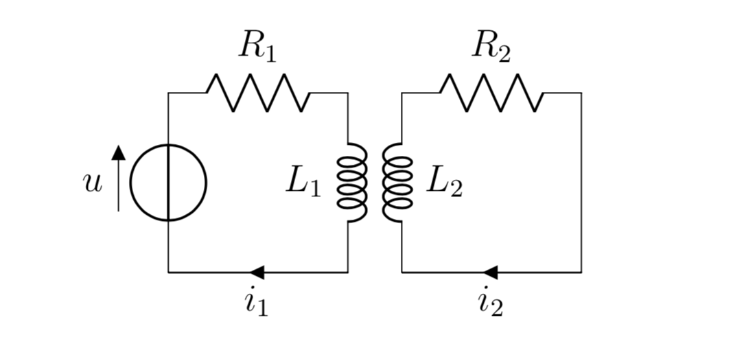
Model of two electrical circuits with currents $i_j$, resistances $R_j$, mutually coupled inductors $L_j$ and a voltage source $u$.
Problem Definition
In general, optimal control problems can be made arbitrarily complex, depending on how the system is described, what constraints the state must fulfill and what we want to optimize for. Here, we will consider the special case where our system of interest is described by a linear ODE
\begin{align}
\dot{x}(t) &= A(t) x(t)+B(t) u(t)\\
x(0) &= x_{0} \in \mathbb{R}^n,
\end{align}
where we assume our control $u$ to take values in $[-1,1]^m$, $A(t) \in \mathbb{R}^{n \times n}$ and $B(t) \in \mathbb{R}^{n \times m}$. Let’s say we want to reach some target state $x_T$ in minimum time, then we need to solve the following problem:
\begin{align}
\tag{P}
& \min
& & t(u) \\
& \text{subject to}
& & x(t(u), u) = x_T
\end{align}
Our illustrative example of two coupled circuits can be described by the above formulation. Let’s say we would like to reach a certain electrical current $i_1$ in the circuit on the left as fast as possible by controlling the voltage source $u$. But, we do not want to induce any current in the circuit on the right once we complete our adjustments to the voltage. The current in both circuits can be expressed as the state of a linear ODE and we can model the situation as a linear time-optimal control problem in the form above.1 But what does such an optimal control look like?
Optimality and the Bang-Bang Principle
One can show that as long as a control $u$ exists such that the final state $x_T$ can be reached, then a time-optimal control also exists. For linear systems one can additionally prove that any state $x_T$ that is attainable in finite time can also be reached by a control with values only in ${-1,1}$. Such a control is called bang-bang. This is a very interesting result since it reduces the search for an optimal control to the search for points where the control switches between $-1$ and $1$. In fact, using some tools from functional analysis one can show that a necessary condition for optimality is that any optimal solution has bang-bang structure. This result is a special case of Pontryagin’s Maximum Principle. If $A$ and $B$ are constant matrices then under certain regularity conditions the optimal control is unique, the number of switches is finite and if all eigenvalues of $A$ are real then this number is even bounded by $n-1$! So we can prove a lot about the structure of optimal controls, but how do we actually go about finding one in practice? In order to do this we turn to numerical methods.
Numerical Solution
We will solve the linear time-optimal control problem numerically by transforming it into a finite-dimensional non-linear optimization problem. To achieve this we consider a discrete-time grid and the state, control and objective are approximated by a suitable discretization. This approach is called a direct method.
Discretization
We begin by using a trick in order to transform our problem to the interval $[0,1]$ in order to have a fixed interval which to discretize. Then we can formulate an equivalent problem for $(t,u)$. Suppose now we have an approximation $(u^k)_k$ of the control variable. We can obtain the discretized state $(x^k)_k$ by using any numerical integration method (e.g. Runge-Kutta methods). This leads to the following non-linear optimization problem:
\begin{align}
\tag{NLP}
& \min
& & t \\
& \text{subject to}
& & t \in [0,\infty) \\
&
& & u^{k} \in [-1,1]^m \quad k = 1,\dots,r\\
&
& & x^{r} = x_T
\end{align}
We can now use standard methods from non-linear optimization to solve this problem.
Optimization
We will compare two methods for solving optimization problems with nonlinear equality constraints and box constraints in an attempt to solve (NLP). Both rely on introducing a term to the objective function which substitutes the equality constraints. This results in a box-constrained optimization problem which can then be solved efficiently for example by specialized interior-point or active set methods. Suppose we would like to solve the following optimization problem
\begin{align}
& \min
& & f(u) \\
& \text{subject to}
&& g(u) = 0.
\end{align}
The Quadratic Penalty Method relies on the idea of moving complicated constraints into the objective function and penalizing a deviation from them. For a penalty parameter $c > 0$ the penalty function
\begin{equation} L_c(u,0) = f(u) + \frac{c}{2} {\lVert g(u) \rVert}^2 \end{equation}
is optimized. This is done iteratively while increasing the penalty parameter and replacing the initial guess by the solution of the previous iteration. Unfortunately, even a global minimum to the penalty function does not necessarily have to be feasible for the original constrained problem. In practice however, the penalty method generally converges at least to a local optimum of the original problem. Another issue with the penalty method is, that for large $c$ the problem becomes ill-conditioned. This can be seen very easily when using a Newton-type algorithm, since the condition number of the Hessian $\nabla^2 L_{c}(u,0)$ increases with $c$.
Another method to solve the problem above is the Augmented Lagrangian Method. It additionally introduces an approximation to the Lagrange multiplier into the objective function
\begin{equation} L_{c}(u,\lambda) = f(u) + \lambda^{\top} g(u) + \frac{c}{2} {\lVert g(u) \rVert}^2. \end{equation}
We can interpret this as solving a box-constrained optimization problem with the Lagrangian function as the objective by the penalty method. The crucial difference to the penalty method is that we can avoid its ill-conditioning since by the introduction of the approximation to the Lagrange multiplier $c$ does not need to be increased as much. To illustrate this behaviour we computed solutions to a simple test problem called the rocket car problem.
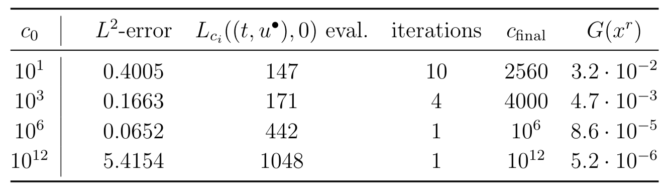
Behavior of the penalty method for different initial penalty coefficients $c_0$ on the rocket car problem.
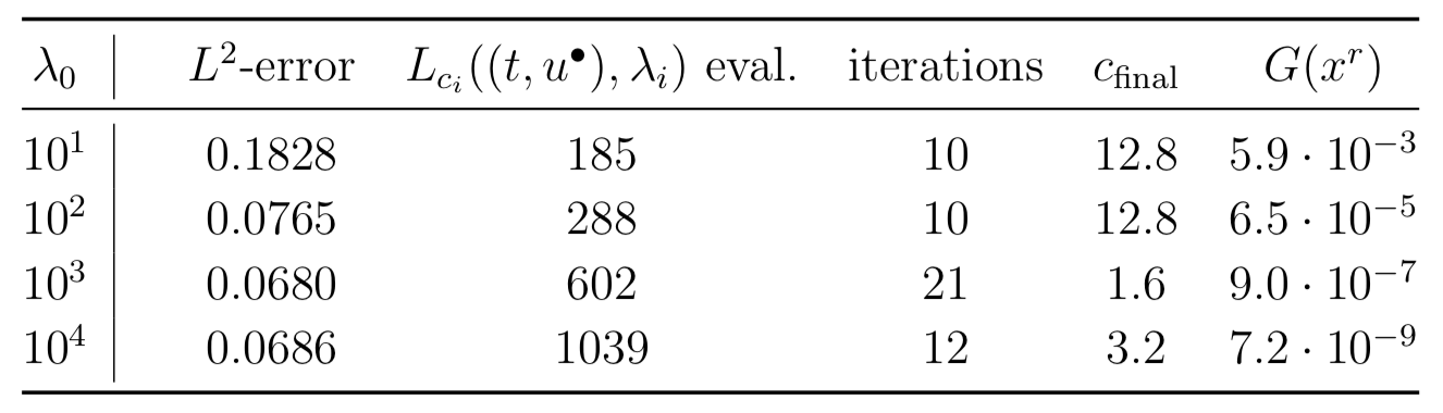
Behavior of the augmented Lagrangian method for fixed initial penalty coefficient $c_0=0.1$ and different initial approximations (\lambda_0) to the Lagrange multiplier on the rocket car problem.
We can clearly see the aforementioned ill-conditioning of the quadratic penalty method for large $c$. Somewhat surprisingly the number of function evaluations is not significantly higher for the augmented Lagrangian method even though it takes more iterations to converge. We can also compare the two methods with respect to the error when using finer and finer discretizations. This is shown in the next figure.
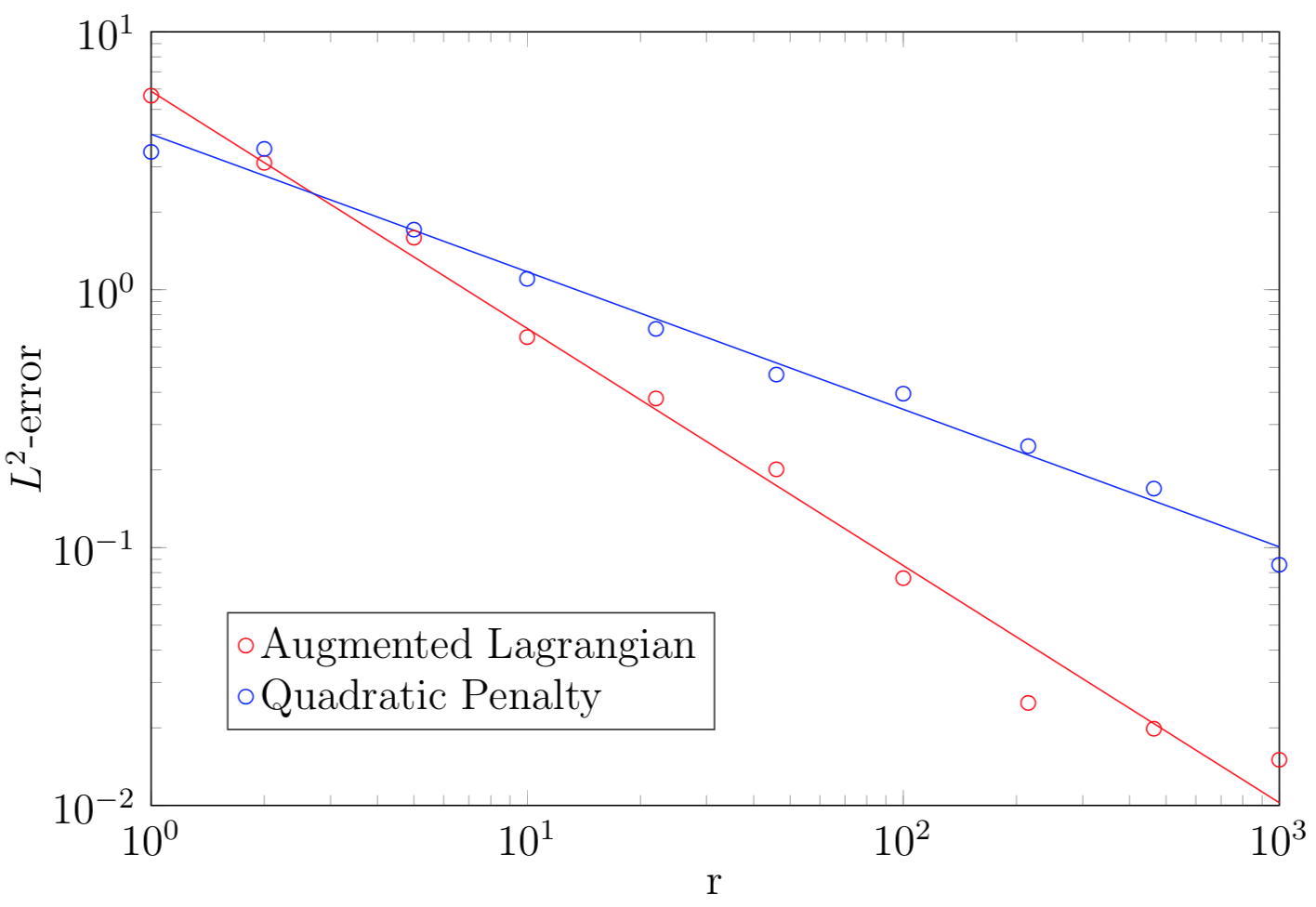
Logarithmic plot of the $L^2$-error between the analytic solution and computed approximations on the discrete-time grid $0 < \frac{1}{r} < \frac{2}{r} < \dots < \frac{r-1}{r}< 1$ for $r \in \mathbb{N}$
In general, as exemplified by this toy problem the augmented Lagrangian method is preferrable to the quadratic penalty method for the linear time-optimal control problem, since it avoids ill-conditioning and performs comparably well both in respect to accuracy and computation time.
Gradient Computation
In order to speed up the optimization procedures we can supply an expression for the computation of the gradient instead of relying on a finite-difference approximation. One can approach this in two ways. Either, we compute the gradient to the discretized problem or we compute the derivative of the continuous problem using the concept of a Fréchet derivative and then discretize. This is a choice that often has to be made when solving problems like these numerically. Surprisingly, in the case of the linear time-optimal control problem these two expressions actually coincide! The order of discretization and differentiation does not matter here.
Time-optimal Control of the Heat Equation
Lastly, we will look at a common application where linear time-optimal control problems naturally arise. A control problem with dynamics described by a linear partial differential equation can be rewritten as a linear time-optimal control problem, when discretized spatially first. Here we will consider the transient heat equation, which describes the heat distribution in a region over time in the presence of a heat or cooling source.
\begin{align}
\partial_t \varphi - \Delta \varphi &= f\mbox{,}\\
\varphi(\cdot,0) &= \varphi_0
\end{align}
By introducing a spatial grid with step length $h$ and discretizing the Laplace operator by a finite difference scheme we obtain
\begin{align}
\partial_t \varphi_h - A_h \varphi_h &= B_hu,\\
\varphi_h(0) &= \varphi_{h0},
\end{align}
where the discretized Laplacian2 is given by
\begin{equation}
A_h =
\frac{1}{h^2}
\begin{bmatrix}
-2 & 1\\
1 & -2 & 1\\
& & \ddots&\\
& & 1 & -2 & 1\\
& & & 1 & -2
\end{bmatrix} \in \mathbb{R}^{n \times n}\mbox{.}
\end{equation}
Assume now we wish to steer this system to a desired heat configuration in minimum time, then we need to solve a problem of type (P). An illustration of the state and computed time-optimal control for a given initial heat configuration on the unit interval is given below.
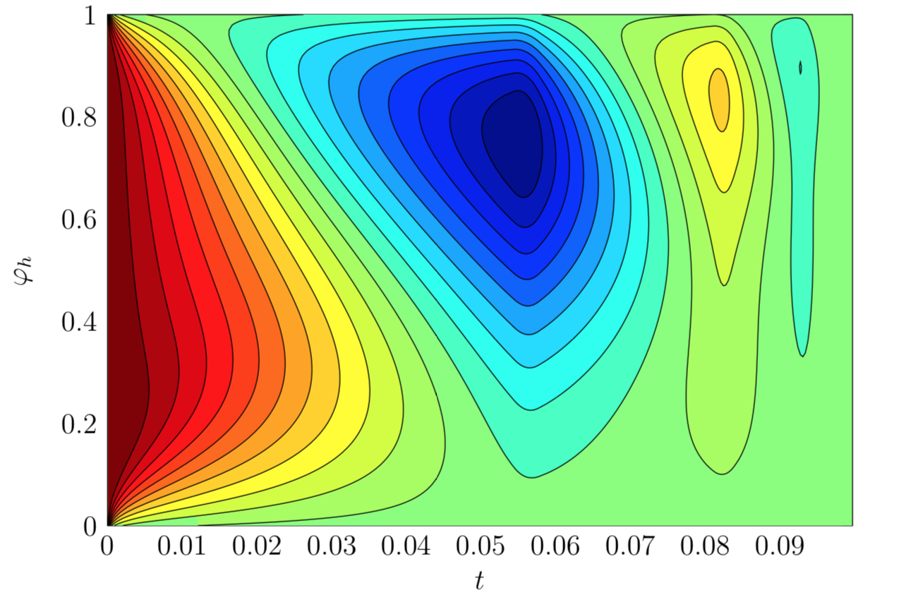
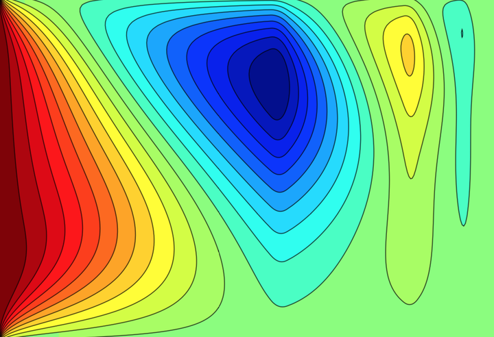
Illustration of the state $\varphi_h$ of the discretized transient heat equation on the unit interval $[0,1]$ over time under the influence of a time-optimal control steering the system to uniform zero heat.
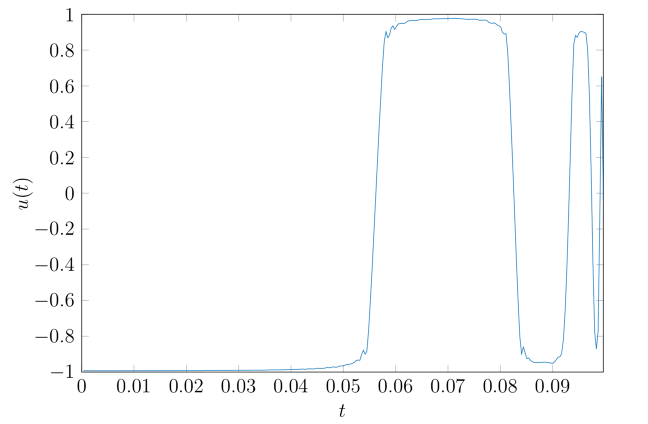
Plot of the computed time-optimal control $u$ steering the system described by the discretized transient heat equation on the unit interval $[0, 1]$ to uniform zero heat.
- Altmann, K., Stingelin, S., and Tröltzsch, F. (2014). On some optimal control problems for electrical circuits. International Journal of Circuit Theory and Applications, 42(8):808–830. ^
- LeVeque, R. (2007). Finite Difference Methods for Ordinary and Partial Differential Equations: Steady-State and Time-Dependent Problems. Society for Industrial and Applied Mathematics (SIAM) ^